Integrating computer vision systems into enterprise operations requires a shift in engineering philosophy from experimental model development to robust, systems-level architecture. While training a deep learning model to high accuracy within a software notebook represents an important initial milestone, building a production-grade system demands reliable, end-to-end data pipelines, optimized hardware acceleration, system-level monitoring, and scalable infrastructure.
The engineering approach of FNA Technology bypasses traditional agency bloat by placing senior practitioners directly at the helm of design and system engineering. This structural paradigm ensures that deep learning models do not remain isolated demonstrations, but instead operate as integrated, high-throughput components within broader enterprise software architectures.
To bridge the gap between pilot studies and industrial-scale execution, computer vision architectures must be designed to withstand real-world variables, including shifting environmental conditions, computational resource constraints, and data-drift phenomena. Since 2023, FNA Technology has delivered over 25 major production-grade products globally across key regions including India, the United States, Singapore, the United Arab Emirates, and the United Kingdom, achieving a 5/5 client rating. Key production deployments include platforms such as Akeed and Khedmah. The structural systems, execution parameters, and deployment methodologies described in this report outline a comprehensive blueprint for constructing reliable, production-ready computer vision applications across diverse edge and cloud environments.
Technical Lifecycle and Scoping Architecture
The lifecycle of an enterprise computer vision solution is a continuous, structured engineering cycle divided into five key phases: Discovery, Design, Build, Launch, and Support. By maintaining a model of direct access to senior engineers and completely eliminating account management layers or rotating juniors, architectural decisions are grounded in technical reality from day one.
During the initial Discovery phase, the engineering team maps the target business metrics to concrete technical requirements. This phase focuses heavily on assessing data availability, as this dictates the model training pipeline. If representative custom data is not readily available, the architecture is designed around pre-trained foundation models or synthetic data generation tools, whereas prediction or classification models require custom training pools.
The Design phase translates physical constraints into validated software layouts, incorporating UX research and component-based UI design systems. The Build phase implements the core machine learning models, accelerated inference graphs, and backend pipelines. Launch executes production-ready deployments via automated CI/CD tracks. Finally, the Support phase establishes ongoing performance monitoring under strict Service Level Agreements (SLAs) and coordinates retraining loops as new production data is acquired.
| Lifecycle Phase | Core Technical Deliverables | Typical Duration | Scoping Metrics & Scenarios |
|---|---|---|---|
| Discovery | Architecture mapping, data audit, and integration planning | 1 – 2 Weeks | Scoped by data availability, target accuracy bar, and API constraints |
| Design | Figma assets, interactive click-prototypes, and design tokens | 2 – 4 Weeks | Validated layouts mapped to software engineering realities |
| Build | Model training, Triton configurations, and edge pipeline setup | 4 – 8 Weeks | Scaled by model parameters, edge optimization targets, and pipeline steps |
| Launch | Container deployment, integration testing, and release staging | 1 – 2 Weeks | Verified against accuracy benchmarks and API latency limits |
| Support | SLAs, performance tuning, data drift alerts, and retraining loops | Ongoing | Retraining triggered by visual embedding drift detections |
While conversational interfaces and fine-tuned large language models can be integrated into production environments within 2 to 4 weeks, custom computer vision pipelines requiring full data collection, deep training, and physical edge evaluation operate on a 2-to-4-month production trajectory. Scoping parameters factor in the complexity of existing database integrations, camera network protocols, and target hardware environments.
Data-Centric MLOps and Active Curation Pipelines
The long-term performance of computer vision systems deployed in production is directly tied to the data pipelines that feed them. Rather than executing bulk manual annotations—which incur high costs and yield diminishing statistical returns—the pipeline utilizes Active Learning (AL) algorithms to identify high-value data points for annotation.
Active Learning and Embeddings Curation
To execute active learning, the system ingests raw camera or video streams and processes them through an embedding engine, such as LightlyStudio or FiftyOne, to extract high-dimensional vector representations. Cosine similarity is computed across these vectors to evaluate spatial and semantic relationships. The similarity metric is defined as:
By mapping these visual embeddings, the system implements the ALPHA clustering-based active sampling framework. This algorithm clusters visually redundant frames, isolates the centroids of these semantic clusters, and propagates annotations across the visual cluster neighborhood, eliminating redundant labeling efforts on highly similar data.
Furthermore, during live inference, the pipeline monitors model prediction uncertainty, such as class confidence scores residing near the decision boundary. It also tracks visual embedding drift, identifying frames that exhibit features structurally divergent from the training distribution. These flagged frames are automatically routed into an active learning queue to generate a specialized dataset targeting edge-case failure modes, such as severe lighting changes, physical occlusions, or camera misalignments.
Immutable Data Versioning and Drift Response
Reproducibility in deep learning requires strict alignment between code, model weights, and the exact data partitions utilized during training. The data pipeline implements Data Version Control (DVC) alongside metadata layers to version evaluation sets as immutable, Git-traceable artifacts.
Once deployed, the live model's input feature distributions are continuously analyzed. The system monitors covariate drift—the shifting of input image distributions over time—by training a binary classifier to distinguish between the training baseline dataset and real-world production frames. A significant increase in this auxiliary classifier’s performance indicates that production data has drifted, which automatically triggers alert mechanisms and initiates the active learning ingestion loop to dynamically update and retrain the primary models.
Intelligent Video Analytics at the Edge
Executing real-time inference on multi-stream high-definition video feeds requires maximizing physical hardware performance and minimizing CPU-GPU memory copy overhead. This is achieved by building optimized graph architectures using the open-source GStreamer framework and the NVIDIA DeepStream SDK.
Hardware-Accelerated Pipeline Architecture
The video analytics pipeline is constructed as a directed acyclic graph of modular, hardware-accelerated GStreamer plugins. Within this architecture, frame data remains inside GPU memory (represented as NvMM memory blocks) throughout the entire processing cycle, preventing costly Host-to-Device (CPU-to-GPU) memory transfers.
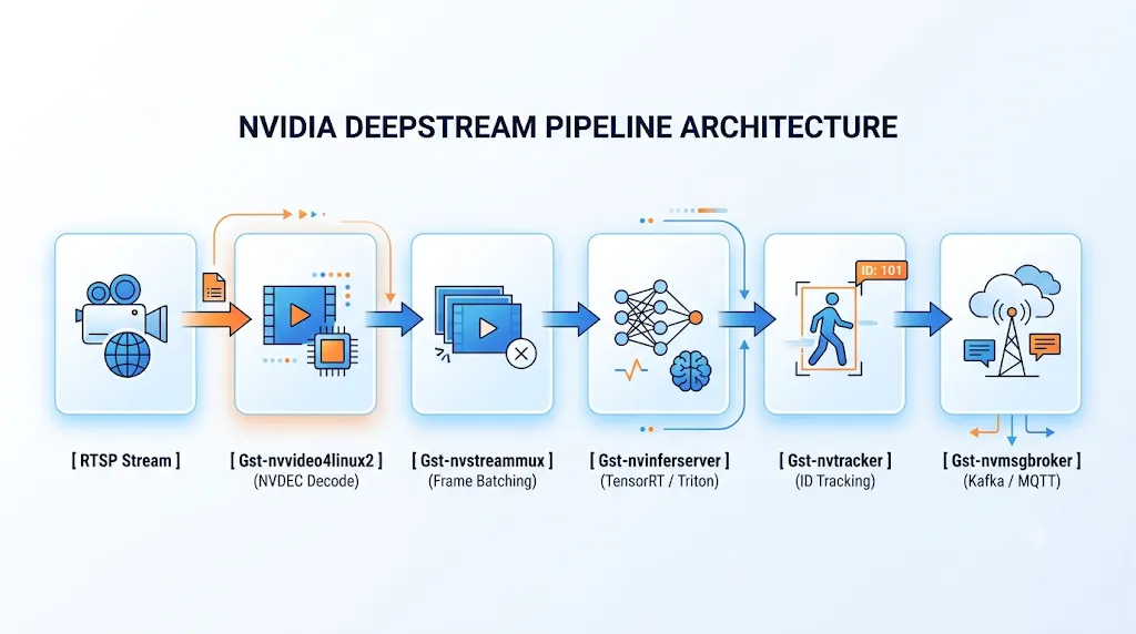
First, incoming RTSP camera streams are ingested and hardware-decoded using the NVDEC accelerator via the Gst-nvvideo4linux2 plugin. The decoded frames undergo spatial resizing, scaling, and color space conversion (e.g., from YUV to RGBA) using the Vision Image Compositor (VIC) or dedicated GPU hardware through the Gst-nvvideoconvert plugin.
Individual frames from multiple camera streams are then aggregated into structured, synchronized batches using the Gst-nvstreammux plugin, maximizing GPU tensor core utilization during the downstream inference stage. Deep learning inference is performed using either native TensorRT compiled engines via Gst-nvinfer or concurrently managed multi-framework backends via the Gst-nvinferserver plugin, which integrates the NVIDIA Triton Inference Server directly into the streaming pipeline. To maintain spatial-temporal consistency, the Gst-nvtracker plugin assigns persistent tracking IDs to detected bounding boxes, utilizing highly optimized trackers such as KLT or DeepSORT implementations.
Every GStreamer buffer flowing through the graph carries an attached, custom metadata structure named NvDsBatchMeta. This structure progressively accumulates inference results, bounding box coordinates, class labels, and tracking IDs from upstream plugins. Finally, the pipeline serializes model outputs into structured JSON schemas utilizing the Gst-nvmsgconv plugin, which are subsequently published to cloud endpoints or local message brokers via Kafka, MQTT, or AMQP protocols using the Gst-nvmsgbroker plugin, facilitating real-time alerting and integration with external enterprise systems.
Hardware-Level Offloading and Acceleration
Deploying to resource-constrained edge appliances, such as the NVIDIA Jetson Orin series, necessitates offloading specific operations away from CUDA cores and the CPU host.
| Hardware Component | Pipeline Function | DeepStream Plugin | Computational Benefit |
|---|---|---|---|
| NVDEC | Hardware-accelerated video decoding | Gst-nvvideo4linux2 | Bypasses host CPU, preventing frame drop during ingestion |
| VIC / PVA | Color conversion, scaling, and dewarping | Gst-nvvideoconvert | Saves CUDA GPU cores for actual deep learning model execution |
| DLA Core | Independent neural network acceleration | Gst-nvinfer | Executes secondary models (e.g. classification) on specialized silicon |
| CUDA Core | High-throughput tensor mathematics | Gst-nvinferserver | Runs primary transformers and complex spatial-temporal models |
| NVENC | Outbound video stream encoding | Gst-nvvenc | Encodes annotated streams for low-latency RTSP rebroadcasting |
By maintaining raw video buffers strictly within GPU memory spaces (NvMM), the CPU's role is restricted to basic stream orchestration and OS-level metadata routing. This architectural design achieves near-zero CPU utilization overhead, enabling a single edge computer to simultaneously decode, track, and analyze up to 16 high-definition camera feeds.
Object Detection Benchmarks: RT-DETR vs. YOLO
Selecting the appropriate object detection model requires evaluating the fundamental architectural trade-offs between Convolutional Neural Networks (CNNs) and Vision Transformers (ViTs) under strict real-time execution constraints.
Architectural Philosophies and the NMS Bottleneck
Historically, the YOLO (You Only Look Once) family of models has dominated real-time visual detection. However, traditional one-stage anchor-based or anchor-free CNN detectors must employ Non-Maximum Suppression (NMS) as a post-processing step to filter out overlapping candidate bounding boxes. The execution time of NMS is highly non-deterministic and scales quadratically () relative to the density of detected objects within a scene. This introduces variable latency spikes and hampers predictable real-time performance on edge devices.
RT-DETR (Real-Time Detection Transformer) resolves this bottleneck by treating object detection as an end-to-end set prediction task. Using a hybrid encoder to process multi-scale features and a transformer decoder with uncertainty-minimal query selection, RT-DETR directly outputs a fixed set of non-overlapping bounding boxes. This architectural design eliminates NMS post-processing entirely, ensuring a highly deterministic latency profile.
The modern YOLO family, specifically YOLO11 and the newer YOLO26, has countered this transformer transition by introducing native end-to-end NMS-free CNN designs (originating from YOLOv10 architectures). YOLO26 leverages a specialized MuSGD optimizer and structured loss formulations (such as ProgLoss and STAL loss functions) to improve spatial convergence speeds and small-object detection without introducing the massive memory footprint characteristic of transformer backbones.
Quantitative Performance Matrix
| Model Variant | Base Architecture | Param Count | GFLOPs | mAP50-95 | TensorRT FP16 Latency | Primary Engineering Fit |
|---|---|---|---|---|---|---|
| YOLO11n | CNN | ~2.6M | ~6.5 | 38.9% | ~1.5 ms | Ultra-low power edge devices, microcontrollers |
| YOLO11x | Optimized CNN | 56.9M | 194.9 | 54.7% | 11.3 ms | High-accuracy real-time manufacturing and edge inspection |
| RT-DETR-R50 | Hybrid ViT | 42.0M | 136.0 | 53.1% | 9.2 ms (108 FPS) | Dense, highly occluded scenes (e.g., retail queue tracking) |
| RT-DETR-R101 | Hybrid ViT | 76.0M | 259.0 | 54.3% | 13.5 ms (74 FPS) | High-end GPU servers with complex global spatial contexts |
| YOLO26x | NMS-Free CNN | ~51.0M | ~181.0 | 55.2% | 10.1 ms | Deterministic low-latency targets with tight memory budgets |
Note: All inference benchmarks are evaluated at a standard spatial input resolution of 640 × 640 pixels.
YOLO11 and YOLO26 represent the optimal design choice for highly constrained edge systems lacking substantial CUDA memory or running on CPU-only hosts, where their compact CNN kernels achieve rapid convergence and a minimal physical footprint. RT-DETR is the superior solution for high-density environments (such as crowded urban spaces or dense warehousing logistics) where spatial occlusions are prevalent. The global receptive field provided by its self-attention mechanism excels at mapping contextual relationships across distant regions of the frame.
Zero-Shot Video Segmentation with SAM 2
The introduction of the Segment Anything Model 2 (SAM 2) has redefined promptable video object tracking and rotoscoping. Rather than training highly specialized, single-class segmenters, SAM 2 operates as a foundation model capable of segmenting any object across space and time based on minimal user prompts (such as a single coordinate point, bounding box, or mask input).
The Streaming Memory Mechanism
SAM 2 extends zero-shot static image segmentation into the temporal video domain by integrating an on-chip streaming memory architecture.
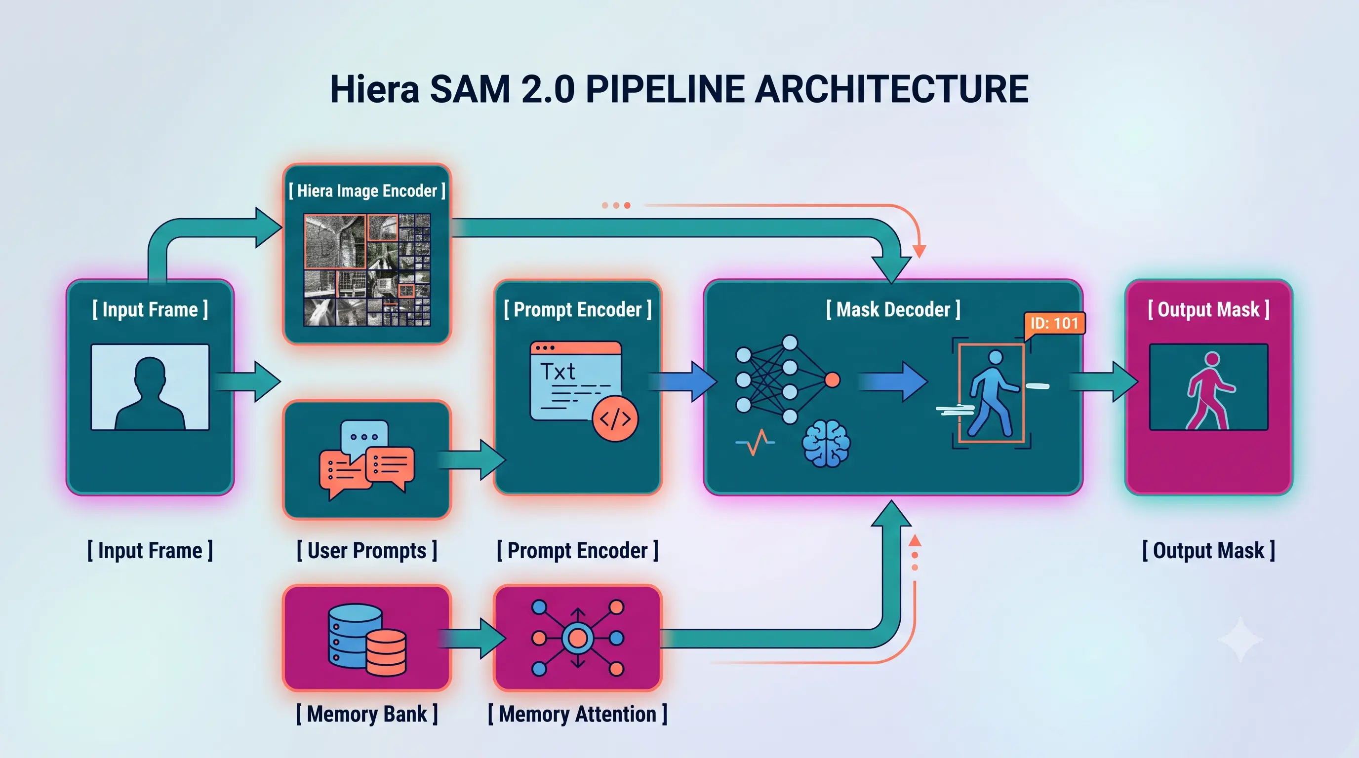
The memory encoder compresses the predicted mask and visual features into a compact, low-dimensional spatial representation. The memory bank maintains a queue of historical frame embeddings, storing detailed spatial information from the most recent frames, alongside sparse, long-term temporal context representations from ancestral frames. The memory attention layer, implemented as a series of transformer blocks, performs cross-attention between current frame features and the historical representations in the memory bank. This mechanism ensures that the model preserves structural knowledge of the target object's geometry, compensating for radical changes in scale, severe lighting variations, and prolonged object occlusions.
Optimization Profiles across Model Scales
| Model Scale | Parameter Count | mAP (SA-V) | FP16 Throughput (NVIDIA A100) | Orin AGX (64GB) Target | Optimal Target Environment |
|---|---|---|---|---|---|
| Tiny | 38.9M | 75.0% | ~91 FPS | ~12 FPS | Resource-constrained edge platforms, Jetson devices |
| Small | 46.0M | 74.9% | ~85 FPS | ~10 FPS | Edge appliances with mid-range processing budgets |
| Base+ | 80.8M | 74.7% | ~64 FPS | ~6 FPS | Production cloud workloads, real-time tracking |
| Large | 224.4M | 76.0% | ~30 FPS | ~2 FPS | High-fidelity offline rotoscoping, medical imagery |
To run the SAM 2 model on edge processors like the Jetson Orin Nano, the model must be split into modular components—specifically, the Image Encoder, Memory Attention, Prompt Encoder, and Mask Decoder—which are individually exported to ONNX format and compiled into high-performance TensorRT engines using FP16 quantization. Without this localized TensorRT compilation, executing the Python-based PyTorch framework directly on edge platforms yields extremely slow processing speeds (~1 FPS), rendering it unusable for real-time video streaming.
Intelligent Document Processing: Layout-Aware Multimodal Systems
Modern Document AI systems have evolved from basic Optical Character Recognition (OCR) systems into multimodal comprehension platforms. These systems process unstructured paperwork (such as financial invoices, regulatory submissions, or logistics waybills) directly into structured, searchable database schemas.
LayoutLMv3 vs. Donut: Comparative Methodology
Building an Intelligent Document Processing (IDP) pipeline requires choosing between two distinct multimodal paradigms:
LayoutLMv3 (Multimodal OCR-First)
A multimodal transformer that unifies text, visual layout, and raw image features in a single, multi-stream architecture. The model receives extracted text tokens from an initial OCR processor alongside corresponding spatial bounding box coordinates normalized to a 0–1000 coordinate system. Simultaneously, the source document image is segmented into visual patches.
This approach is highly accurate and provides precise spatial coordinates for downstream auditability, but its performance is heavily bound by the quality of the upstream OCR engine.
Donut (OCR-Free Seq2Seq)
An end-to-end, OCR-free Document Understanding Transformer. It employs a visual Swin Transformer encoder to extract feature representations directly from raw page pixels, coupled with a BART-style generative text decoder that outputs structured JSON strings directly.
By bypassing the OCR step entirely, Donut avoids cascading OCR errors. However, generative decoding is computationally expensive, requires high-end GPUs, and cannot natively output exact spatial coordinates.
| Feature Dimension | LayoutLMv3 | Donut |
|---|---|---|
| Input Modality | Raw Image + OCR Tokens + Spatial Bounds | Raw Document Image Only (Pixels) |
| Architecture | Multimodal Multi-Stream Encoder-Only | Seq2Seq (Swin Encoder + BART Decoder) |
| Output Target | Token-level class labels (e.g., BIO tags) | Serialized structured JSON string |
| OCR Dependency | Yes (e.g., DocTR, Tesseract) | No (completely OCR-free end-to-end) |
| Spatial Provenance | Excellent (maintains exact spatial coordinates) | None (relies on text-generation order) |
Microservice-Based IDP Architecture
To scale document processing pipelines to handle thousands of pages hourly, the system isolates high-latency, GPU-bound processes behind dedicated microservices.
Step 1: Hybrid Classification. When a multi-page document is received, it is split into individual page images. To minimize API costs, a hybrid classification routing strategy is deployed. A local, zero-cost CLIP-KNN classifier maps the page image into embedding space and matches it against an indexed library of known document layouts. If the local classifier's confidence score drops below a pre-configured threshold (), the page is routed to a Vision-Language Model (VLM), such as Claude 3.5 Sonnet, to resolve the layout. This hybrid approach achieves near-VLM accuracy while reducing API costs by approximately 90%.
| Classification Strategy | Accuracy | Average Latency per Page | API Cost per 1,000 Pages |
|---|---|---|---|
| CLIP-KNN Only | 92% | 0.5 – 1.0 s | $0.00 |
| VLM Only (Claude Sonnet) | 98% | 2.0 – 3.0 s | $10.00 |
| Hybrid Strategy (4% Fallback) | 96% | 0.6 – 1.2 s | $0.40 |
Step 2: Auxiliary Spatial Metadata Extraction. For documents requiring strict verification (e.g., validating physical signatures or scanning barcodes), an object detection model like RF-DETR is executed over localized regions of interest.
Step 3: OCR and Text Stitching. The page image is processed using a two-stage OCR pipeline to extract word-level coordinates and raw text strings. Individual page outputs are stitched into a coherent, structured document representation.
Step 4: Structured Field Parsing. The stitched document representation, along with its layout metadata, is processed by a parser to extract final structured fields. The parsing step employs either structured LLMs (using Pydantic validation schemas via the Instructor framework) or fine-tuned multimodal encoders to write the output data directly into the target database.
Integration Topologies and Ecosystem Cohesion
The value of custom computer vision pipelines is realized when they are integrated directly into enterprise applications. Rather than operating as isolated models, vision pipelines connect via secure APIs, webhooks, or high-throughput database pipelines to adjacent software environments.
| Target System | Protocol | Typical Bandwidth | Latency Window | Core Architecture Match |
|---|---|---|---|---|
| Next.js Web Portal | WebSocket, REST API | Low to Moderate (JSON payloads) | 20 – 50 ms | Real-time object tracking and operational alerting |
| Native iOS / Android App | Local CoreML / NNAPI | Zero (Internal edge execution) | < 15 ms | On-device face verification or active gesture control |
| Enterprise Cloud Database | Encrypted PostgreSQL | Low (Structured data inserts) | 100 – 200 ms | IDP extraction pipeline archiving or analytics |
| Cloud Object Store | HTTPS / S3 API | High (Archiving raw image frames) | Asynchronous | Hard-example active learning storage |
Rigorous Safety, Accuracy, and Evaluation Frameworks
Production deployment requires rigorous performance validation before any model update is staged. To establish high reliability, the system implements automated evaluation frameworks to continuously test models against specific business and safety benchmarks.
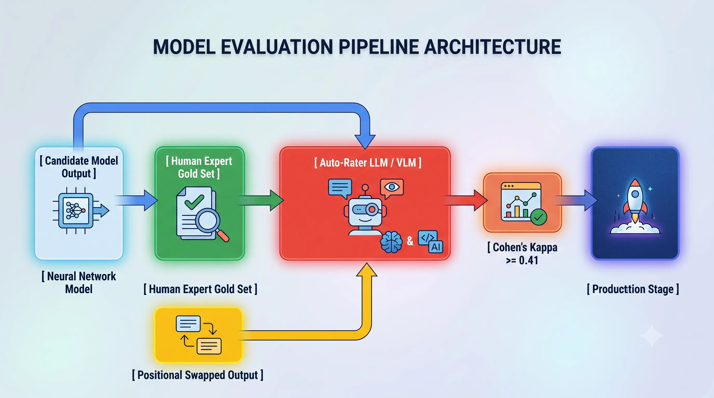
For large-scale classification or semantic extraction tasks, the engineering team implements automated rater mechanisms (VLM/LLM-as-a-Judge) to grade model predictions against a human-validated gold standard dataset. To eliminate positional bias—where generative raters favor specific output structures or display orderings—the evaluation pipeline executes systematic Positional Swaps on input candidates during evaluation.
The alignment between the automated auto-rater and verified human experts is measured using Cohen's Kappa () coefficient:
where represents the relative observed agreement among raters, and is the hypothetical probability of chance agreement. Model updates are only staged for production release when the evaluation pipeline achieves a kappa score of , verifying moderate-to-high statistical agreement with human domain experts.
Once verified, models are launched using canary release patterns to monitor live performance and prevent regressions. Post-launch telemetry tracking then feeds data back into the active learning loop, establishing a continuous cycle of retraining and optimization.
Build Production AI with FNA Technology
FNA Technology designs, builds, and deploys intelligent systems entirely in-house. Our engineering studio works directly with startup, SME, and enterprise leaders to ship high-performance computer vision architectures globally.